Case 3: Benchmark and Method validation

In this example, we show how to compare the results from implicit and explicit H-bond methods.

Import the required packages

import os

import prolif as plf
from prolif import sdf_supplier
from prolif.io.protein_helper import ProteinHelper
from prolif.molecule import Molecule
from prolif.plotting.complex3d import Complex3D
from rdkit import Chem

/home/yuyang/Project_local/GSoC2025_Hbond_PM/.venv/lib/python3.11/site-packages/MDAnalysis/topology/tables.py:52: DeprecationWarning: Deprecated in version 2.8.0
MDAnalysis.topology.tables has been moved to MDAnalysis.guesser.tables. This import point will be removed in MDAnalysis version 3.0.0
  warnings.warn(wmsg, category=DeprecationWarning)

# custom functions for comparison and plotting
from validation.utils.metrics import (
    confusion_matrix,
    get_interactions,
    plot_confusion_matrix,
    tanimoto_coefficient_by_confusion_matrix,
)

We also use the protein helper function to read the files.

protein_helper = ProteinHelper(
    templates=[
        {
            "MSE": {"SMILES": "C[Se]CC[CH](N)C=O"},
        }
    ]
)

The test case is from PLINDER: 5da9__1__1.A_1.B__1.E_1.F. We have prepared the protonated file in the repository.

test_case_dir = "./test_data/5da9__1__1.A_1.B__1.E_1.F"

Explicit H-bond method

First, we read the molecule from the path.

protein_mol = Molecule.from_rdkit(
    Chem.MolFromPDBFile(
        f"{test_case_dir}/receptor_protonated.pdb",
        sanitize=False,
        removeHs=False,
        proximityBonding=True,
    )
)
protein_mol = protein_helper.standardize_protein(protein_mol)

Then, we check the length of the residues.

protein_mol.residues.__len__()

834

We also check with the residues to know whether they are fixed with our protein helper as expected.

plf.display_residues(protein_mol, slice(0, 10), sanitize=False)

We next load all ligands in the directory.

ligands = []
for ligand_sdf in os.listdir(test_case_dir):  # noqa: PTH208
    if ligand_sdf.endswith("_protonated.sdf"):
        ligands.extend(sdf_supplier(f"{test_case_dir}/{ligand_sdf}"))

There are two ligands in our directory.

ligands

[<prolif.molecule.Molecule with 1 residues and 47 atoms at 0x7fb4128bb3d0>,
 <prolif.molecule.Molecule with 1 residues and 1 atoms at 0x7fb4129c3510>]

plf.display_residues(ligands[0])

We currently focus on the cation/anion one.

ligand = ligands[0]

Then, we calculate the H-bond interactions (using explicit hydrogens).

fp = plf.Fingerprint(["HBDonor", "HBAcceptor"], count=True)
fp.run_from_iterable([ligand], protein_mol, progress=False)
df = fp.to_dataframe().T

Here is the result.

df

		Frame	0
ligand	protein	interaction
UNL1	ARG13.A	HBAcceptor	1
	ASN36.A	HBAcceptor	1
	GLY37.A	HBAcceptor	1
	GLY39.A	HBAcceptor	1
	LYS40.A	HBAcceptor	1
	THR41.A	HBAcceptor	1
	THR42.A	HBAcceptor	1
	ALA64.A	HBDonor	1
	ASP68.A	HBAcceptor	1
	GLN159.A	HBAcceptor	1
	ARG431.A	HBAcceptor	1
	GLY344.B	HBAcceptor	1
	GLN345.B	HBAcceptor	1

2D visualization

We visualize the result into an 2D plot.

view = fp.plot_lignetwork(ligand, kind="frame", frame=0, display_all=False)
view

3D visualization

The result can also be visualized in 3D plot.

view = fp.plot_3d(ligand, protein_mol, frame=0, display_all=True)
view

3Dmol.js failed to load for some reason. Please check your browser console for error messages.

<prolif.plotting.complex3d.Complex3D at 0x7fb4128211d0>

Implicit H-bond method

To have a better comparison, we simply remove the hydrogens from the object instead of reading a new file without explicit hydrogens.

protein_mol_i = protein_helper.standardize_protein(
    Molecule.from_rdkit(Chem.RemoveAllHs(protein_mol))
)

Again, we check the residues after our protein helper.

plf.display_residues(protein_mol_i, slice(0, 10), sanitize=False)

Same for the ligand, we remove the hydrogens.

ligand_i = Molecule.from_rdkit(Chem.RemoveAllHs(ligand))

We then can recalculate the H-bond interations (but with implicit hydrogens).

fp_i = plf.Fingerprint(
    ["ImplicitHBDonor", "ImplicitHBAcceptor"],
    count=True,
)
fp_i.run_from_iterable([ligand_i], protein_mol_i, progress=False)
df_i = fp_i.to_dataframe().T

Here is the result.

df_i

		Frame	0
ligand	protein	interaction
UNL1	ARG13.A	ImplicitHBAcceptor	1
	ASN36.A	ImplicitHBAcceptor	1
	GLY37.A	ImplicitHBDonor	1
		ImplicitHBAcceptor	1
	SER38.A	ImplicitHBDonor	1
		ImplicitHBAcceptor	2
	GLY39.A	ImplicitHBAcceptor	1
	LYS40.A	ImplicitHBDonor	1
		ImplicitHBAcceptor	2
	THR41.A	ImplicitHBAcceptor	3
	THR42.A	ImplicitHBAcceptor	2
	ALA64.A	ImplicitHBDonor	1
	ASP68.A	ImplicitHBAcceptor	1
	SER342.B	ImplicitHBDonor	1
		ImplicitHBAcceptor	1
	GLY344.B	ImplicitHBAcceptor	1
	GLN345.B	ImplicitHBAcceptor	1

2D visualization

view = fp_i.plot_lignetwork(ligand_i, kind="frame", display_all=False)
view

3D visualization

view = fp_i.plot_3d(ligand_i, protein_mol_i, frame=0, display_all=True)
view

3Dmol.js failed to load for some reason. Please check your browser console for error messages.

<prolif.plotting.complex3d.Complex3D at 0x7fb412a73150>

Comparison between explicit and implicit H-bond methods

For the 3D visualization, we can plot the results side by side using compare function. The left panel shows the H-bond interations from explicit hydrogens and the right panel is those from implicit hydrogens.

# create Complex3D objects (left: explicit)
comp3D = Complex3D.from_fingerprint(fp, ligand, protein_mol, frame=0)
# (right: implicit)
other_comp3D = Complex3D.from_fingerprint(fp_i, ligand_i, protein_mol_i, frame=0)

# compare the two Complex3D objects
view = comp3D.compare(other_comp3D, display_all=True)
view

3Dmol.js failed to load for some reason. Please check your browser console for error messages.

<prolif.plotting.complex3d.Complex3D at 0x7fb4128b0a90>

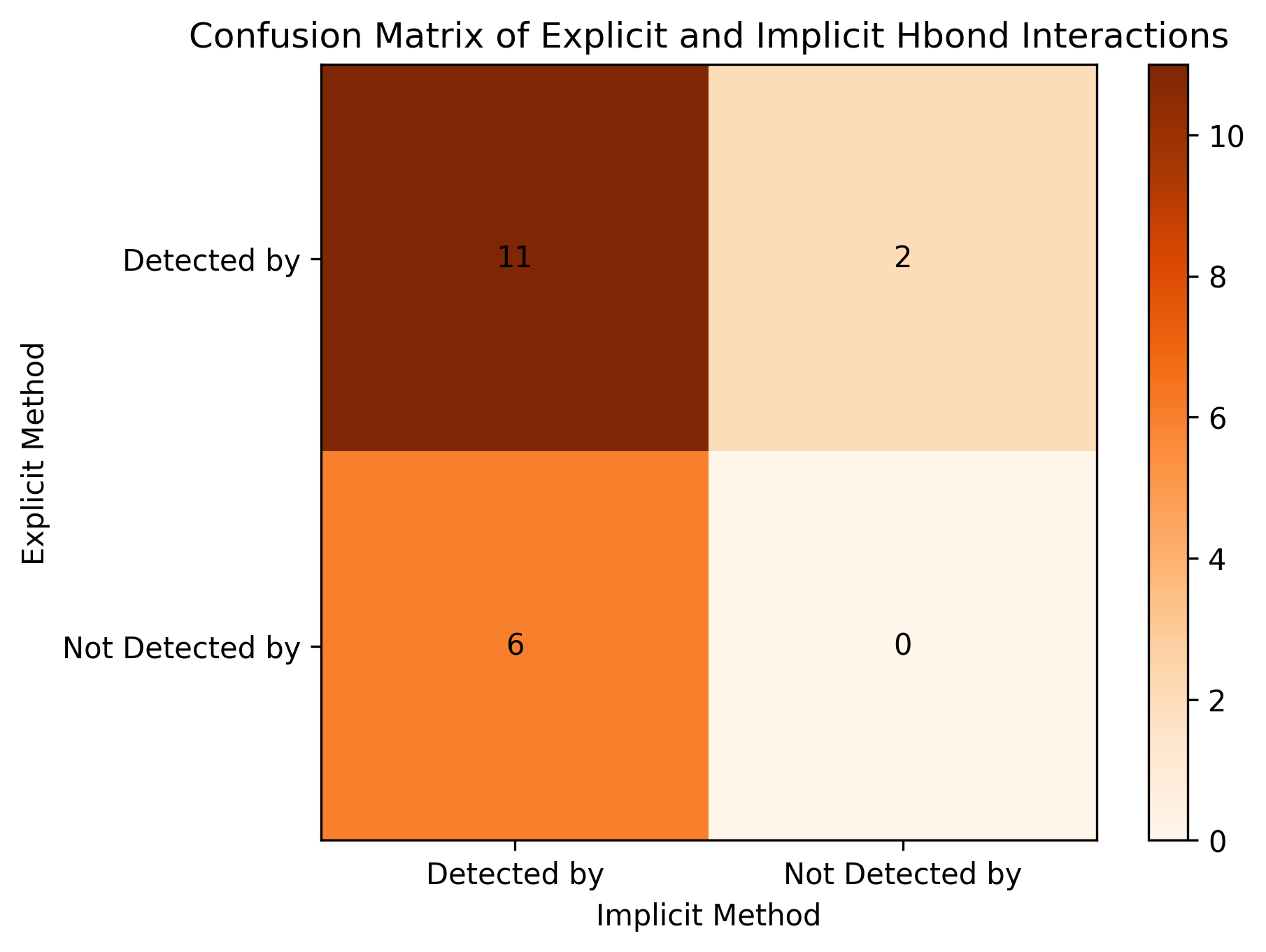
For the interation pairs, we can covert the result into two sets explicit_set and implicit_set. Then, we can know how many interactions detected by the explicit H-bond method overlap with those detected by the implicit H-bond method.

explicit_set = get_interactions(df)
implicit_set = get_interactions(df_i)

matrix = confusion_matrix(explicit_set, implicit_set)
tm_coef = tanimoto_coefficient_by_confusion_matrix(matrix)

The Tanimoto coefficient (also called intersection over union) is a measure used to evaluate performance. A higher score indicates better performance.

print("Tanimoto coefficient:", tm_coef)  # noqa: T201
fig, ax = plot_confusion_matrix(matrix)
fig.show()

Tanimoto coefficient: 0.5789473684210527